How to bulk download data from Google Trends using Python
Google trends is a website by Google that analyses the popularity of searches made on Google over time. It can be a very useful tool for numerous applications such as digital marketing or market research but anyone who wants to make deeper analyses will find the process cumbersome as the platform is not targeted at analysts who needs lot of data.
On top of that, the way scores are calculated is not made public by Google. Rather, the company explains it provides a normalized index based on the absolute search volume and the timeframe.
As a result, scores may vary based on the set of keywords and timeframes requested. Therefore, queries should be made one at the time with the same timeframe in order to compare them.
In this article, we will see how we can bulk download queries and save them in a CSV file using Python, Jupyter notebook and the Pytrends API.
Installation
If you don’t have the API, just type !pip install pytrends at the beginning of your notebook. You can then delete the cell as you need to install it only once.
1. Import libraries
Start by importing the needed libraries. We need Pytrends obviously, pandas to store the data in dataframes and time to add some waiting time beetween queries.
2. Connect to Google
To request data from Google Trends, we need to import the TrendReq method from Pytrends.
The method has the following parameters:
hl: host language
tz: timezone
retries: number of retries
We will use english and the standard GMT timezone. The latter is more important when you look for hourly trends, which is not the case here. More info on all available parameters can be find on the Pytrends page.
3. Keywords and geographic locations
We can now create two lists with the keywords and locations we are interested in.
Countries have to be in the two letter abbreviations format.
You can also look for trends in particular regions. Unfortunately, there is no list of codes for regions online. The best way to find them is to to do a generic query on the Google trends platform, clic on the country/region you are interested in and look at the geo term in the URL.
For example, Paris is FR-J (https://trends.google.com/trends/explore?date=all&geo=FR-J&q=food).
4. Build a query loop
We will now create a loop that makes a query for each of the combinations of keywords and locations. Each result will be stored in a multilevel dictionary.
Google errors: Google often return errors. It can be either because the keyword does not bring sufficient searches on Google in that particular location or because you make too many queries at the server.
In order to tackle the second scenario, we add a sleeping time between each queries with the variable wait and store all unsucessful queries into a separate list that we will use later.
The loop
It will tell you the number of queries to do, print each one of them that was unsuccessful and tell you once it is done.
Tackle errors
After all queries have been made, we can look again for all unsuccessful ones multiple times. This allows us to minimize the number of errors that happened for other reasons than no data available.
The loop tells you the number of queries to do, how many loops it has done and the remaining unsuccessful queries.
Save dataframe and CSV file
Now that we made all our queries and are confident we got all the available data, we can convert the results in a dataframe and save it as a CSV file.
5. Create a function
We can also take the whole code and create a function named googletrends_queries() that takes as arguments the keywords list keywords, the locations list geo and the number of loops to do with the unsuccessful queries.
To use the function, you just have to run it with the existing lists as parameters. The CSV file will be saved during the function as trends.csv by default. You can also save the results in a dataframe and continue with your analysis:
In case the waiting time is too long for you, you can modify it when calling the function by defining the wait parameter. For ex: googletrends_queries(keywords=keywords, geo=geo, loops=1, wait=1)
6. Output
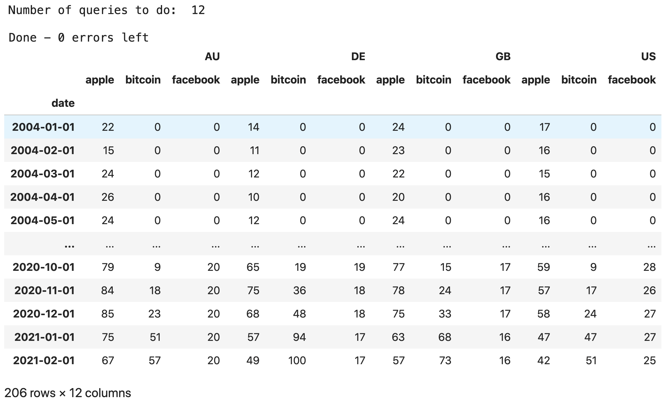
Using keywords=[‘apple’, ‘facebook’, ‘bitcoin’] and geo=[‘US’, ‘AU’, ‘GB’, ‘DE’], we get the following output:
The multilevel dataframe contains the 204 monthly average trends for the 3 keywords we looked for in the 4 countries. Not so much interest for Facebook or Bitcoin back in 2004 :)
In a following post, we will see how to best visualize this data in Python using Plotly.
I hope this will help anyone starting with Google trends and trying to gather bulk data. Have fun and bear in mind that sometimes the Google trends server is capricious and returns only errors. In such case, just try later.
